Loss functions

Loss functions are used to quantify how well or bad a model can reproduce the values of the training set.

The appropriate loss function depends on the type of problems and the algorithm we use.

Let's denote with $\hat y$ the prediction of the model and $y$ the true value.

Gaussian noise

Let's assume that the relationship between the features $X$ and the label $Y$ is given by

$$ Y = f(X) +\epsilon$$

where $f$ is the model whose parameters we want to fix and $\epsilon$ is some random noise with zero mean and variance $\sigma$.

The likelihood to measure $y$ for feature values $x$ is given by

$$L\sim \exp\left(-\frac{(y-f(x))^2}{2\sigma}\right) $$

If we have a set of examples $x^{(i)}$ the likelihood becomes

$$ L\sim \prod_i \exp\left(-\frac{(y^{(i)}-f(x^{(i)}))^2}{2\sigma}\right) $$

We now want to fix the parameters in $f$ such that we maximize the likelihood that our data was generated by the model.

It is more convenient to work with the log of the likelihood. Maximizing the likelihood is equivalent to minimising the negative log-likelihood.

$$ NLL = - \log(L) = \frac{1}{2\sigma} \sum_i \left(y^{(i)}-f(x^{(i)})\right)^2 $$

So assuming gaussian noise for the difference between the model and the data leads to the least square rule.

We can use the square error loss

$$ J(f) = \sum_i \left(y^{(i)}-f(x^{(i)})\right)^2 $$

To train our machine learning algorithm.

Two class model

If we have two classes, we call one the positive class ($c=1$) and the other the negative class ($c=0$). If the probability to belong to class 1

$$p(c=1) = p$$

we also have

$$ p(c=0)=1-p $$

The likelihood for a single measurement if the outcome is in the positive class is $p$ and if the outcome is in the negative class the likelihood is $1-p$. For a set of measurements with outcomes $y_i$ the likelihood is given by

$$ L = \prod\limits_{y_i=1} p \prod\limits_{y_i=0} (1-p) $$

So the negative log-likelihood is:

$$ NLL = - \sum\limits_{y_i=1} \log(p) - \sum\limits_{y_i=0} \log(1-p) $$

Given that $y=0$ or $y=1$ we can rewrite it as

$$ NLL = - \sum \left( y \log(p) + (1-y)\log(1-p) \right) $$

So if we have a model for the probability $\hat y = p(X)$ we can maximize the likelihood of the training data by optimizing

$$ J= - \sum_i y_i \log \left(\hat y\right) +(1-y_i)\log\left(1 - \hat y\right) $$

It is called the cross entropy.

Perceptron loss

One can formulate the perceptron algorithm in terms of a stochastic gradient descent with the loss given by

$$ J(w) = \sum h( y_i p(x_i,w))$$

where $p(x_i,w)$ is the model prediction $\vec x\cdot \vec w + w_0$ and $h$ is the hinge function:

$$ h(x)=\left\{ \begin{array}{ccc} -x & \mbox{if} & x < 0 \\ 0 &\mbox{if}& x \ge 0 \end{array}\right. $$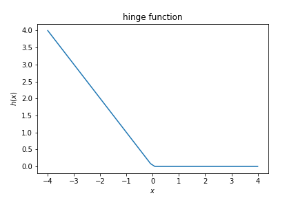

Support vector machine

The loss for the SVM also uses the hinge function, but offset such that we penalise values up to 1:

$$ J(w) = \frac{1}{2}\vec w\cdot \vec w + C \sum h_1( y_i p(x_i,w)) $$

where $p(x_i,w)$ is the model prediction $\vec x\cdot \vec w + w_0$ and $h_1$ is the shifted hinge function.

$$ h_1(x) = \max(0, 1- x).$$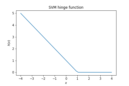

$C$ is a model parameter controlling the trade-off between the width of the margin and the amount of margin violation.